gftool.lattice.honeycomb.dos_mp
- gftool.lattice.honeycomb.dos_mp(eps, half_bandwidth=1)[source]
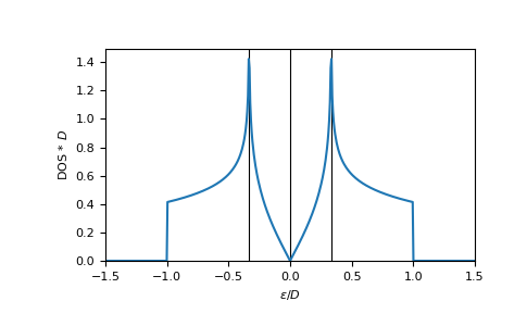
Multi-precision DOS of non-interacting 2D honeycomb lattice.
The DOS diverges at eps=±half_bandwidth/3.
This function is particularity suited to calculate integrals of the form \(∫dϵ DOS(ϵ)f(ϵ)\). If you have problems with the convergence, consider removing singularities, e.g. split the integral
\[∫^0 dϵ DOS(ϵ)[f(ϵ) - f(-D/3)] + ∫_0 dϵ DOS(ϵ)[f(ϵ) - f(+D/3)] + [f(-D/3) + f(+D/3)]/2\]where \(D\) is the half_bandwidth, or symmetrize the integral.
The Green’s function and therefore the DOS of the 2D honeycomb lattice can be expressed in terms of the 2D triangular lattice
gftool.lattice.triangular.dos_mp, see [horiguchi1972].- Parameters:
- epsmpmath.mpf or mpf_like
DOS is evaluated at points eps.
- half_bandwidthmpmath.mpf or mpf_like
Half-bandwidth of the DOS, DOS(| eps | > half_bandwidth) = 0. The half_bandwidth corresponds to the nearest neighbor hopping \(t=2D/3\).
- Returns:
- mpmath.mpf
The value of the DOS.
See also
gftool.lattice.honeycomb.dosVectorized version suitable for array evaluations.
gftool.lattice.triangular.dos_mp
References
[horiguchi1972]Horiguchi, T., 1972. Lattice Green’s Functions for the Triangular and Honeycomb Lattices. Journal of Mathematical Physics 13, 1411-1419. https://doi.org/10.1063/1.1666155
Examples
Calculated integrals
>>> from mpmath import mp
>>> mp.quad(gt.lattice.honeycomb.dos_mp, [-1, -1/3, 0, +1/3, +1])
mpf('1.0')
>>> eps = np.linspace(-1.5, 1.5, num=501)
>>> dos_mp = [gt.lattice.honeycomb.dos_mp(ee, half_bandwidth=1) for ee in eps]
>>> import matplotlib.pyplot as plt
>>> for pos in (-1/3, 0, +1/3):
...     _ = plt.axvline(pos, color='black', linewidth=0.8)
>>> _ = plt.plot(eps, dos_mp)
>>> _ = plt.xlabel(r"$\epsilon/D$")
>>> _ = plt.ylabel(r"DOS * $D$")
>>> _ = plt.ylim(bottom=0)
>>> _ = plt.xlim(left=eps.min(), right=eps.max())
>>> plt.show()