gftool.lattice.kagome.gf_z
- gftool.lattice.kagome.gf_z(z, half_bandwidth)[source]
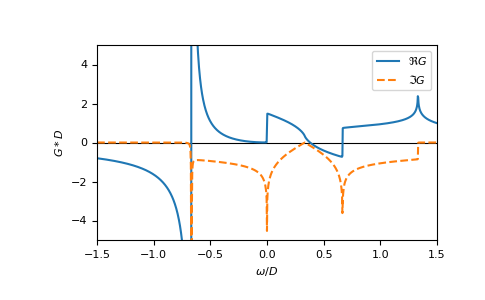
Local Green’s function of the 2D kagome lattice.
The Green’s function of the 2D kagome lattice can be expressed in terms of the 2D triangular lattice
gftool.lattice.triangular.gf_z, and a non-dispersive peak, see [kogan2021]. Omitting the non-dispersive peak, it corresponds togftool.lattice.honeycomb.gf_zshifted by half_bandwidth/3.The Green’s function has singularities for z/half_bandwidth in [-2/3, 0, 2/3].
- Parameters:
- zcomplex np.ndarray or complex
Green’s function is evaluated at complex frequency z.
- half_bandwidthfloat
Half-bandwidth of the DOS of the kagome lattice. The half_bandwidth corresponds to the nearest neighbor hopping \(t=2D/3\).
- Returns:
- complex np.ndarray or complex
Value of the kagome lattice Green’s function.
See also
References
[varm2013]Varma, V.K., Monien, H., 2013. Lattice Green’s functions for kagome, diced, and hyperkagome lattices. Phys. Rev. E 87, 032109. https://doi.org/10.1103/PhysRevE.87.032109
[kogan2021]Kogan, E., Gumbs, G., 2020. Green’s Functions and DOS for Some 2D Lattices. Graphene 10, 1-12. https://doi.org/10.4236/graphene.2021.101001
Examples
>>> ww = np.linspace(-1.5, 1.5, num=1001, dtype=complex) + 1e-4j
>>> gf_ww = gt.lattice.kagome.gf_z(ww, half_bandwidth=1)
>>> import matplotlib.pyplot as plt
>>> _ = plt.axhline(0, color='black', linewidth=0.8)
>>> _ = plt.plot(ww.real, gf_ww.real, label=r"$\Re G$")
>>> _ = plt.plot(ww.real, gf_ww.imag, '--', label=r"$\Im G$")
>>> _ = plt.ylabel(r"$G*D$")
>>> _ = plt.xlabel(r"$\omega/D$")
>>> _ = plt.xlim(left=ww.real.min(), right=ww.real.max())
>>> _ = plt.ylim(bottom=-5, top=5)
>>> _ = plt.legend()
>>> plt.show()
