gftool.beb.solve_root

gftool.beb.solve_root(z, e_onsite, concentration, hopping, hilbert_trafo: Callable[[complex], complex], self_beb_z0=None, restricted=True, rcond=None, **root_kwds)

Determine the BEB self-energy by solving the root problem.

Note, that the result should be checked, whether the obtained solution is physical.

Parameters:

z(…) complex np.ndarray

Frequency points.

e_onsite(…, N_cmpt) float or complex np.ndarray

On-site energy of the components.

concentration(…, N_cmpt) float np.ndarray

Concentration of the different components.

hopping(N_cmpt, N_cmpt) float array_like

Hopping matrix in the components.

hilbert_trafoCallable[[complex], complex]

Hilbert transformation of the lattice to calculate the local Green’s function.

self_beb_z0(…, N_cmpt, N_cmpt) complex np.ndarray, optional

Starting guess for the BEB self-energy.

restrictedbool, optional

Whether the diagonal of self_beb_z is restricted to self_beb_z.imag <= 0 (default: True). Note, that even if restricted=True, the imaginary part can get negative within tolerance. This should be removed by hand if necessary.

rcondfloat, optional

Cut-off ratio for small singular values of hopping. For the purposes of rank determination, singular values are treated as zero if they are smaller than rcond times the largest singular value of hopping.

**root_kwds

Additional arguments passed to scipy.optimize.root. method can be used to choose a solver. options=dict(fatol=tol) can be specified to set the desired tolerance tol.

Returns:

(…, N_cmpt, N_cmpt) complex np.ndarray

The BEB self-energy as the root of self_root_eq.

Raises:

RuntimeError

If the root problem cannot be solved.

See also

gf_loc_z

Notes

The root problem is solved for the complete input simultaneously. This provides a speed up as the code is vectorized, however, it comes with the trade-off of complicating the root search. So in some cases, it makes sense to split the input arrays, and calculate the root separately.

The default method is ‘krylov’, which typically does a good job. In some cases ‘excitingmixing’ was found to do a better job, especially close to the CPA limit, where some singular values become small.

The progress of the root search is logged for the logging.DEBUG level.

Examples

>>> from functools import partial
>>> eps = np.array([-0.5, 0.5])
>>> c = np.array([0.3, 0.7])
>>> t = np.array([[1.0, 0.3],
...               [0.3, 1.2]])
>>> hilbert = partial(gt.bethe_hilbert_transform, half_bandwidth=1)

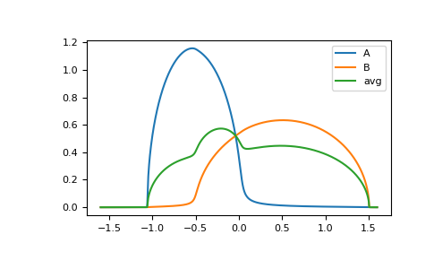
>>> ww = np.linspace(-1.6, 1.6, num=1000) + 1e-4j
>>> self_beb_ww = gt.beb.solve_root(ww, e_onsite=eps, concentration=c, hopping=t,
...                                 hilbert_trafo=hilbert)
>>> gf_loc_ww = gt.beb.gf_loc_z(ww, self_beb_ww, hopping=t, hilbert_trafo=hilbert)

>>> import matplotlib.pyplot as plt
>>> __ = plt.plot(ww.real, -1./np.pi/c[0]*gf_loc_ww[:, 0].imag, label='A')
>>> __ = plt.plot(ww.real, -1./np.pi/c[1]*gf_loc_ww[:, 1].imag, label='B')
>>> __ = plt.plot(ww.real, -1./np.pi*np.sum(gf_loc_ww.imag, axis=-1), label='avg')
>>> __ = plt.legend()
>>> plt.show()

(png, pdf)