gftool.cpa.solve_root
- gftool.cpa.solve_root(z, e_onsite, concentration, hilbert_trafo: Callable[[complex], complex], self_cpa_z0=None, restricted=True, **root_kwds)[source]
Determine the CPA self-energy by solving the root problem.
Note that the result should be checked, whether the obtained solution is physical.
- Parameters:
- z(…) complex array_like
Frequency points.
- e_onsite(…, N_cmpt) float or complex np.ndarray
On-site energy of the components. This can also include a local frequency dependent self-energy of the component sites.
- concentration(…, N_cmpt) float array_like
Concentration of the different components used for the average.
- hilbert_trafoCallable[[complex], complex]
Hilbert transformation of the lattice to calculate the coherent Green’s function.
- self_cpa_z0(…) complex np.ndarray, optional
Starting guess for CPA self-energy.
- restrictedbool, optional
Whether self_cpa_z is restricted to self_cpa_z.imag <= 0. (default: True) Note, that even if restricted=True, the imaginary part can get negative within tolerance. This should be removed by hand if necessary.
- **root_kwds
Additional arguments passed to
scipy.optimize.root. method can be used to choose a solver. options=dict(fatol=tol) can be specified to set the desired tolerance tol.
- Returns:
- (…) complex np.ndarray
The CPA self-energy as the root of
self_root_eq.
- Raises:
- RuntimeError
If unable to find a solution.
Notes
For restricted=True root-serach, we made good experince with the methods ‘anderson’, ‘krylov’ and ‘df-sane’. For restricted=False, we made made good experince with the method ‘broyden2’.
Examples
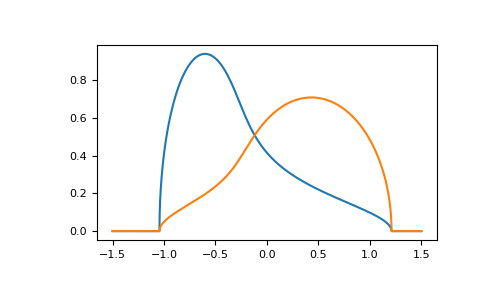
>>> from functools import partial
>>> parameter = dict(
...     e_onsite=[-0.3, 0.3],
...     concentration=[0.3, 0.7],
...     hilbert_trafo=partial(gt.bethe_gf_z, half_bandwidth=1),
... )
>>> ww = np.linspace(-1.5, 1.5, num=5000) + 1e-10j
>>> self_cpa_ww = gt.cpa.solve_root(ww, **parameter)
>>> del parameter['concentration']
>>> gf_cmpt_ww = gt.cpa.gf_cmpt_z(ww, self_cpa_ww, **parameter)
>>> import matplotlib.pyplot as plt
>>> __ = plt.plot(ww.real, -1./np.pi*gf_cmpt_ww[..., 0].imag)
>>> __ = plt.plot(ww.real, -1./np.pi*gf_cmpt_ww[..., 1].imag)
>>> plt.show()
