gftool.beb
Blackman, Esterling, and Berk (BEB) approach to off-diagonal disorder.
It extends CPA allowing for random hopping amplitudes. [blackman1971]
The implementation is based on a SVD of the hopping matrix, which is the dimensionless scaling of the hopping of the components. [weh2021] However, we use the unitary eigendecomposition instead of the SVD.
Physical quantities
The main quantity of interest is the average local Green’s function gf.
First the effective medium self_beb_z has to be calculated using solve_root.
With this result the Green’s function can be calculated by the function gf_loc_z.
In the BEB formalism, the local Green’s function gf is a matrix in the components. The self-consistent Green’s function gf is diagonal, its trace is the average physical Green’s function. If only the non-vanishing diagonal elements have been calculated gf=gf_loc_z(…, diag=True), the average Green’s function is np.sum(gf, axis=-1). The diagonal elements of gf are the average for a specific component (conditional average) multiplied by the concentration of that component.
References
Blackman, J.A., Esterling, D.M., Berk, N.F., 1971. Generalized Locator—Coherent-Potential Approach to Binary Alloys. Phys. Rev. B 4, 2412-2428. https://doi.org/10.1103/PhysRevB.4.2412
Weh, A., Zhang, Y., Östlin, A., Terletska, H., Bauernfeind, D., Tam, K.-M., Evertz, H.G., Byczuk, K., Vollhardt, D., Chioncel, L., 2021. Dynamical mean-field theory of the Anderson–Hubbard model with local and nonlocal disorder in tensor formulation. Phys. Rev. B 104, 045127. https://doi.org/10.1103/PhysRevB.104.045127
Examples
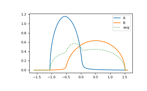
We consider a Bethe lattice with two components ‘A’ and ‘B’. The have the on-site energies -0.5 and 0.5 respectively, the concentrations 0.3 and 0.7. Furthermore, we assume that the hopping amplitude between ‘A’ and ‘B’ is only 0.3 times the hopping between two ‘A’ sites, while the hopping between two ‘B’ sites is 1.2 times the hopping between two ‘A’ sites.
Then the following code calculates the local Green’s function for component ‘A’ and ‘B’ (conditionally averaged) as well as the average Green’s function of the system.
from functools import partial

import gftool as gt
import numpy as np
import matplotlib.pyplot as plt

eps = np.array([-0.5, 0.5])
c = np.array([0.3, 0.7])
t = np.array([[1.0, 0.3],
              [0.3, 1.2]])
hilbert = partial(gt.bethe_hilbert_transform, half_bandwidth=1)

ww = np.linspace(-1.6, 1.6, num=1000) + 1e-4j
self_beb_ww = gt.beb.solve_root(ww, e_onsite=eps, concentration=c, hopping=t,
                                hilbert_trafo=hilbert)
gf_loc_ww = gt.beb.gf_loc_z(ww, self_beb_ww, hopping=t, hilbert_trafo=hilbert)

__ = plt.plot(ww.real, -1./np.pi/c[0]*gf_loc_ww[:, 0].imag, label='A')
__ = plt.plot(ww.real, -1./np.pi/c[1]*gf_loc_ww[:, 1].imag, label='B')
__ = plt.plot(ww.real, -1./np.pi*np.sum(gf_loc_ww.imag, axis=-1), ':', label='avg')
__ = plt.legend()
plt.show()
API
Functions
|
Calculate average local Green's function matrix in components. |
|
Wrap |
|
Root equation r(Σ)=0 for BEB. |
|
Determine the BEB self-energy by solving the root problem. |
Classes
|
SVD like spectral decomposition. |