gftool.polepade

Padé based on robust pole finding.

Instead of fitting a rational polynomial, poles and zeros or poles and corresponding residues are fitted.

The algorithm is based on [ito2018] and adjusted to Green’s functions and self- energies. A very short summary can of the algorithm can be found in the appendix of [weh2020]. We assume that we know exactly the high-frequency behavior of the function we want to continue. Here, we will call it degree and we define it as the behavior of the function f(z) for large abs(z):

\[f(z) ≈ z^{degree}.\]

For the diagonal element’s of the one-particle Green’s function this is degree=-1 for the self-energy it is degree=0.

References

[ito2018]

Ito, S., Nakatsukasa, Y., 2018. Stable polefinding and rational least-squares fitting via eigenvalues. Numer. Math. 139, 633–682. https://doi.org/10.1007/s00211-018-0948-4

[weh2020] (1,2)

Weh, A. et al. Spectral properties of heterostructures containing half-metallic ferromagnets in the presence of local many-body correlations. Phys. Rev. Research 2, 043263 (2020). https://doi.org/10.1103/PhysRevResearch.2.043263

Examples

The function continuation provides a high-level interface which can be used for convenience. Let’s consider an optimal example: We know the Green’s function for complex frequencies on the unit (half-)circle. We consider the Bethe Green’s function.

>>> z = np.exp(1j*np.linspace(np.pi, 0, num=252)[1:-1])
>>> gf_z = gt.bethe_gf_z(z, half_bandwidth=1)
>>> pade = gt.polepade.continuation(z, gf_z, degree=-1, moments=[1])
>>> print(f"[{pade.zeros.size}/{pade.poles.size}]")
[14/15]

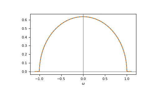
We obtain a [14/15](z) Padé approximant. Let’s compare it on the real axis:

>>> import matplotlib.pyplot as plt
>>> ww = np.linspace(-1.1, 1.1, num=500) + 1e-6j
>>> gf_ww = gt.bethe_gf_z(ww, half_bandwidth=1)
>>> pade_ww = pade.eval_polefct(ww)
>>> __ = plt.axhline(0, color='dimgray', linewidth=0.8)
>>> __ = plt.axvline(0, color='dimgray', linewidth=0.8)
>>> __ = plt.plot(ww.real, -gf_ww.imag/np.pi)
>>> __ = plt.plot(ww.real, -pade_ww.imag/np.pi, '--')
>>> __ = plt.xlabel(r"$\omega$")
>>> plt.show()

(png, pdf)

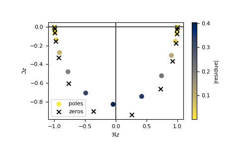
Beside the band-edge, we get a nice fit. We can also investigate the pole structure of the fit:

>>> pade.plot()
>>> plt.show()

(png, pdf)

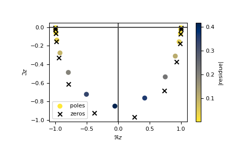
Using a grid on the imaginary axis, the fit is of course worse. Note, that its typically better to continue the self-energy instead of the Green’s function, see appendix of [weh2020]. For more control, instead of using continuation the elementary functions can be used:

number_poles to determine the degree of the Padé approximant
poles, zeros to calculate the poles and zeros of the approximant
residues_ols to calculate the residues

API

Functions

`asymptotic`(z, fct_z, zeros, poles[, weight])	Calculate large z asymptotic from roots and `poles`.
`continuation`(z, fct_z[, degree, weight, ...])	Perform the Padé analytic continuation of (z, fct_z).
`number_poles`(z, fct_z, *[, degree, weight, ...])	Estimate the optimal number of poles for a rational approximation.
`poles`(z, fct_z, *[, n, vandermond, weight])	Calculate position of the m poles.
`residues_ols`(z, fct_z, poles[, weight, moments])	Calculate the residues using ordinary least square.
`zeros`(z, fct_z, poles, *[, n, vandermond, ...])	Calculate position of n zeros given the `poles`.

Classes

PadeApprox(zeros, poles, residues, amplitude)

Representation of the Padé approximation based on poles.