gftool.hermpade
Hermite-Padé approximants from Taylor expansion.
See [fasondini2019] for practical applications and [baker1996] for the extensive theoretical basis.
We present the example from [fasondini2019] showing the approximations.
We consider the cubic root f(z) = (1 + z)**(1/3), the radius of convergence
of its series is 1.
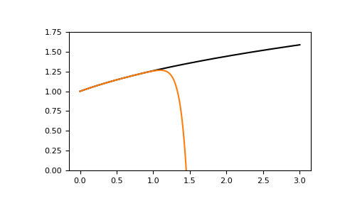
Taylor series
Obviously the Taylor series fails for z<=1 as it cannot represent a pole, but also for larger z>=1 it fails:
>>> from scipy.special import binom
>>> an = binom(1/3, np.arange(17))  # Taylor of (1+x)**(1/3)
>>> def f(z):
...     return np.emath.power(1+z, 1/3)
>>> taylor = np.polynomial.Polynomial(an)
>>> import matplotlib.pyplot as plt
>>> x = np.linspace(0, 3, num=500)
>>> __ = plt.plot(x, f(x), color='black')
>>> __ = plt.plot(x, taylor(x), color='C1')
>>> __ = plt.ylim(0, 1.75)
>>> plt.show()

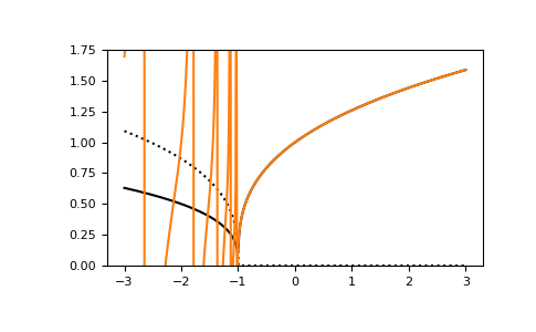
Padé approximant
The Padé approximant can be used to improve the Taylor expansion and expands the applicability beyond the radius of convergence:
>>> x = np.linspace(-3, 3, num=501)
>>> pade = gt.hermpade.pade(an, num_deg=8, den_deg=8)
>>> __ = plt.plot(x, f(x).real, color='black')
>>> __ = plt.plot(x, f(x).imag, ':', color='black')
>>> __ = plt.plot(x, pade.eval(x), color='C1')
>>> __ = plt.ylim(0, 1.75)
>>> plt.show()

The Padé approximant provides a global approximation. For negative values, however, the Padé approximant still fails, as it cannot accurately represent a branch cut. The Padé approximant is suitable for simple poles and tries to approximate the branch-cut by a finite number of poles. It is instructive to plot the error in the complex plane:
>>> y = np.linspace(-3, 3, num=501)
>>> z = x[:, None] + 1j*y[None, :]
>>> error = abs(pade.eval(z) - f(z))
>>> poles = pade.denom.roots()
>>> import matplotlib as mpl
>>> fmt = mpl.ticker.LogFormatterMathtext()
>>> __ = fmt.create_dummy_axis()
>>> norm = mpl.colors.LogNorm(vmin=1e-16, vmax=1)
>>> __ = plt.pcolormesh(x, y, error.T, shading='nearest', norm=norm)
>>> cbar = plt.colorbar(extend='both')
>>> levels = np.logspace(-15, 0, 16)
>>> cont = plt.contour(x, y, error.T, colors='black', linewidths=0.25, levels=levels)
>>> __ = plt.clabel(cont, cont.levels, fmt=fmt, fontsize='x-small')
>>> for ll in levels:
...     __ = cbar.ax.axhline(ll, color='black', linewidth=0.25)
>>> __ = plt.hlines(0, xmin=x[0], xmax=-1, color='red')  # branch cut
>>> __ = plt.scatter(poles.real, poles.imag, color='black', marker='x', zorder=2)  # poles
>>> __ = plt.xlabel(r"$\Re z$")
>>> __ = plt.ylabel(r"$\Im z$")
>>> __ = plt.xlim(x[0], x[-1])
>>> plt.tight_layout()
>>> plt.gca().set_rasterization_zorder(1.5)  # avoid excessive files
>>> plt.show()
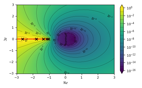
Away from the branch-cut, indicated by the red line, the Padé approximant is a reasonable approximation. The crosses indicate the simple poles of the Padé approximant.
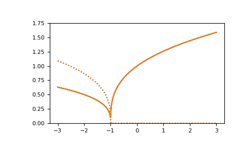
Quadratic Hermite-Padé approximant
A further improvement is provided by the quadratic Hermite-Padé approximant, which can represent square-root branch cuts:
>>> herm2 = gt.hermpade.Hermite2.from_taylor(an, deg_p=5, deg_q=5, deg_r=5)
>>> __ = plt.plot(x, f(x).real, color='black')
>>> __ = plt.plot(x, f(x).imag, ':', color='black')
>>> __ = plt.plot(x, herm2.eval(x + 1e-16j).real, color='C1')
>>> __ = plt.plot(x, herm2.eval(x + 1e-16j).imag, ':', color='C1')
>>> __ = plt.ylim(0, 1.75)
>>> plt.show()

It nicely approximates the function almost everywhere.
However, there is ambiguity which branch to choose, thus we had to add the
shift 1e-16j by hand, to get the correct branch on the real axis.
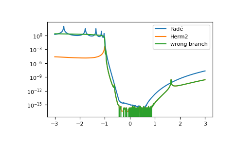
Let’s compare the error to the (linear) Padé approximant:
>>> __ = plt.plot(x, abs(pade.eval(x) - f(x)), label="Padé")
>>> __ = plt.plot(x, abs(herm2.eval(x + 1e-16j) - f(x)), label="Herm2")
>>> __ = plt.plot(x, abs(herm2.eval(x) - f(x)), label="wrong branch")
>>> __ = plt.yscale('log')
>>> __ = plt.legend()
>>> plt.show()

The correct branch nicely approximates the function everywhere, but even the wrong branch performs better than Padé.
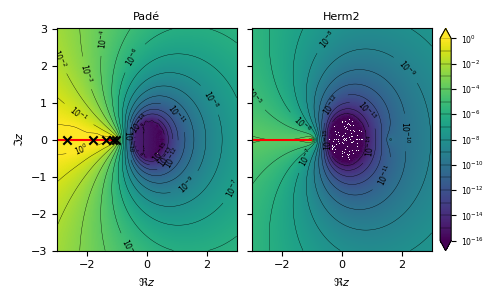
Let’s also compare the quality of the approximants in the complex plane:
>>> error2 = np.abs(herm2.eval(z) - f(z))
>>> __, axes = plt.subplots(ncols=2, sharex=True, sharey=True)
>>> __ = axes[0].set_title("Padé")
>>> __ = axes[1].set_title("Herm2")
>>> levels = np.logspace(-15, 0, 16)
>>> for ax, err in zip(axes, [error, error2]):
...     pcm = ax.pcolormesh(x, y, err.T, shading='nearest', norm=norm)
...     cont = ax.contour(x, y, err.T, colors='black', linewidths=0.25, levels=levels)
...     __ = ax.clabel(cont, cont.levels, fmt=fmt, fontsize='x-small')
...     __ = ax.set_xlabel(r"$\Re z$")
...     __ = ax.hlines(0, xmin=x[0], xmax=-1, color='red')  # branch cut
...     ax.set_rasterization_zorder(1.5)
>>> __ = axes[0].scatter(poles.real, poles.imag, color='black', marker='x', zorder=2)  # poles
>>> __ = plt.xlim(x[0], x[-1])
>>> __ = axes[0].set_ylabel(r"$\Im z$")
>>> plt.tight_layout()
>>> cbar = plt.colorbar(pcm, extend='both', ax=axes, fraction=0.08, pad=0.02)
>>> cbar.ax.tick_params(labelsize='x-small')
>>> for ll in levels:
...     __ = cbar.ax.axhline(ll, color='black', linewidth=0.25)
>>> plt.show()
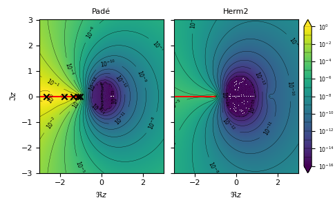
Note, however, the quadratic Hermite-Padé approximant contains the ambiguity which branch to choose. The heuristic can fail and should therefore be checked.
Alternative example: logarithmic branch cut
We also show the results for a logarithmic branch cut, showing that the results
hold not only for algebraic branch cuts.
Let’s consider the approximations for the logarithm f(z) = np.log(1 + z),
whose series has a radius of convergence of 1:
>>> an = np.r_[0, (-1)**np.arange(16)/np.arange(1, 17)]  # Taylor of ln(1+x)
>>> def f(z):
...     return np.emath.log(1 + z)
>>> taylor = np.polynomial.Polynomial(an)
>>> pade = gt.hermpade.pade(an, num_deg=8, den_deg=8)
>>> herm2 = gt.hermpade.Hermite2.from_taylor(an, deg_p=5, deg_q=5, deg_r=5)
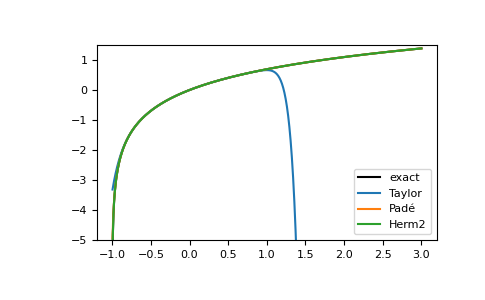
Again, we see that the Taylor series fails for larger z>=1, the (linear) Padé and the quadratic Hermite-Padé, on the other hand, yield good results also for large values.
>>> import matplotlib.pyplot as plt
>>> x = np.linspace(-1, 3, num=1001)[1:]
>>> __ = plt.plot(x, f(x), color='black', label="exact")
>>> __ = plt.plot(x, taylor(x), label="Taylor")
>>> __ = plt.plot(x, pade.eval(x), label="Padé")
>>> __ = plt.plot(x, herm2.eval(x), label="Herm2")
>>> __ = plt.ylim(-5, 1.5)
>>> __ = plt.legend()
>>> plt.show()
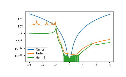
Plotting the error, again we see that the Taylor series is only valid for small values of z, and Padé fails to approximate the branch cut well. The quadratic Hermite-Padé approximant is best for (almost) all values.
>>> x = np.linspace(-3, 3, num=1001)
>>> __ = plt.plot(x, abs(taylor(x) - f(x)), label="Taylor")
>>> __ = plt.plot(x, abs(pade.eval(x) - f(x)), label="Padé")
>>> __ = plt.plot(x, abs(herm2.eval(x) - f(x)), label="Herm2")
>>> __ = plt.yscale('log')
>>> __ = plt.legend()
>>> plt.show()

Plotting the error in the complex plain shows that Padé fails to resolve the branch cut but is else a good approximation globally. The branch-cut is indicated by the red line, the crosses mark the poles of Padé. The Hermite-Padé algorithm yields good results also in the vicinity of the branch cut.
>>> x = np.linspace(-3, 3, num=501)
>>> y = np.linspace(-3, 3, num=501)
>>> z = x[:, None] + 1j*y[None, :]
>>> error = np.abs(pade.eval(z) - f(z))
>>> error2 = np.abs(herm2.eval(z) - f(z))
>>> import matplotlib as mpl
>>> __, axes = plt.subplots(ncols=2, sharex=True, sharey=True)
>>> __ = axes[0].set_title("Padé")
>>> __ = axes[1].set_title("Herm2")
>>> norm = mpl.colors.LogNorm(vmin=1e-16, vmax=1)
>>> for ax, err in zip(axes, [error, error2]):
...     pcm = ax.pcolormesh(x, y, err.T, shading='nearest', norm=norm)
...     cont = ax.contour(x, y, err.T, colors='black', linewidths=0.25, levels=levels)
...     __ = ax.clabel(cont, cont.levels, fmt=fmt, fontsize='x-small')
...     __ = ax.set_xlabel(r"$\Re z$")
...     __ = ax.hlines(0, xmin=x[0], xmax=-1, color='red')  # branch cut
...     ax.set_rasterization_zorder(1.5)
>>> __ = axes[0].scatter(poles.real, poles.imag, color='black', marker='x', zorder=2)  # poles
>>> __ = plt.xlim(x[0], x[-1])
>>> __ = axes[0].set_ylabel(r"$\Im z$")
>>> plt.tight_layout()
>>> cbar = plt.colorbar(pcm, extend='both', ax=axes, fraction=0.08, pad=0.02)
>>> cbar.ax.tick_params(labelsize='x-small')
>>> for ll in levels:
...     __ = cbar.ax.axhline(ll, color='black', linewidth=0.25)
>>> plt.show()
References
Fasondini, M., Hale, N., Spoerer, R. & Weideman, J. A. C. Quadratic Padé Approximation: Numerical Aspects and Applications. Computer research and modeling 11, 1017-1031 (2019). https://doi.org/10.20537/2076-7633-2019-11-6-1017-1031
Baker Jr, G. A. & Graves-Morris, Pade Approximants. Second edition. (Cambridge University Press, 1996).
API
Functions
|
Return the polynomials p, q, r for the quadratic Hermite-Padé approximant. |
|
Return the polynomials p, q, r for the quadratic Hermite-Padé approximant. |
|
Return the [num_deg/den_deg] Padé approximant to the polynomial an. |
|
Return the [num_deg/den_deg] Padé approximant to the polynomial an. |
|
Robust version of Padé approximant to polynomial an. |
Classes
|
Quadratic Hermite-Padé approximant with branch selection according to Padé. |