gftool.linearprediction
Linear prediction to extrapolated retarded Green’s function.
A nice introductory description of linear prediction can be found in [Vaidyanathan2007]; [Makhoul1975] gives a detailed review.
Linear prediction allows to extend a time series by predicting future points \(x̂_l\) as a linear combination of previous time points \(x\):
where \(a_k\) are the prediction coefficients and \(K\) is the
prediction order.
Recommended method to obtain the prediction coefficients is pcoeff_covar,
the results of pcoeff_burg seem to be rather unreliable.
References
Vaidyanathan, P.P., 2007. The Theory of Linear Prediction. Synthesis Lectures on Signal Processing 2, 1-184. https://doi.org/10.2200/S00086ED1V01Y200712SPR003
Makhoul, J. Linear prediction: A tutorial review. Proceedings of the IEEE 63, 561-580 (1975). https://doi.org/10.1109/PROC.1975.9792
Examples
We consider the retarded-time Bethe Green’s function with the known time points
>>> tt = np.linspace(0, 10, 101)
>>> gf_t = gt.lattice.bethe.gf_ret_t(tt, half_bandwidth=1)
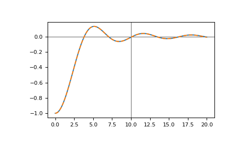
We can predict future time points using linear prediction, let’s check the next 100 time points
>>> lp = gt.linearprediction
>>> pcoeff, __ = lp.pcoeff_covar(gf_t, order=gf_t.size//2)
>>> gf_pred = lp.predict(gf_t, pcoeff, num=100)
and compare the results
>>> import matplotlib.pyplot as plt
>>> tt_pred = np.linspace(0, 20, 201)
>>> gf_full = gt.lattice.bethe.gf_ret_t(tt_pred, half_bandwidth=1)
>>> __ = plt.axhline(0, color='dimgray', linewidth=0.8)
>>> __ = plt.axvline(tt[-1], color='dimgray', linewidth=0.8)
>>> __ = plt.plot(tt_pred, gf_full.imag)
>>> __ = plt.plot(tt_pred, gf_pred.imag, '--')
>>> plt.show()
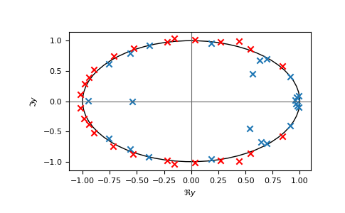
The roots corresponding to the linear prediction polynomial should all lie in the unit circle, numerical inaccuracies can lead to roots outside the unit circle causing exponentially growing contributions. For example, if we add some noise:
>>> noise = np.random.default_rng(0).normal(scale=1e-6, size=tt.size)
>>> pcoeff, __ = lp.pcoeff_covar(gf_t + noise, order=gf_t.size//2)
>>> __ = lp.plot_roots(pcoeff)

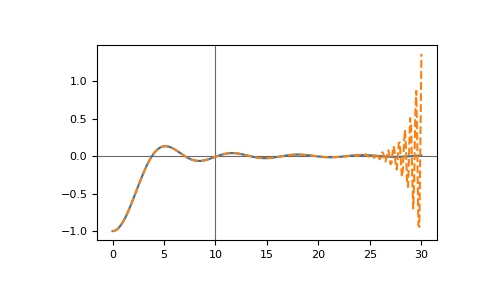
The red crosses correspond to growing contributions. Prediction for long times produces exponentially growing errors:
>>> import matplotlib.pyplot as plt
>>> tt_pred = np.linspace(0, 30, 301)
>>> gf_full = gt.lattice.bethe.gf_ret_t(tt_pred, half_bandwidth=1)
>>> gf_pred = lp.predict(gf_t, pcoeff, num=200)
>>> __ = plt.axhline(0, color='dimgray', linewidth=0.8)
>>> __ = plt.axvline(tt[-1], color='dimgray', linewidth=0.8)
>>> __ = plt.plot(tt_pred, gf_full.imag)
>>> __ = plt.plot(tt_pred, gf_pred.imag, '--')
>>> plt.show()

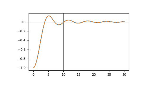
This can be amended by setting stable=True in predict:
>>> import matplotlib.pyplot as plt
>>> tt_pred = np.linspace(0, 30, 301)
>>> gf_full = gt.lattice.bethe.gf_ret_t(tt_pred, half_bandwidth=1)
>>> gf_pred = lp.predict(gf_t, pcoeff, num=200, stable=True)
>>> __ = plt.axhline(0, color='dimgray', linewidth=0.8)
>>> __ = plt.axvline(tt[-1], color='dimgray', linewidth=0.8)
>>> __ = plt.plot(tt_pred, gf_full.imag)
>>> __ = plt.plot(tt_pred, gf_pred.imag, '--')
>>> plt.show()

API
Functions
|
Create a companion matrix. |
|
Burg's method for linear prediction (LP) coefficients. |
|
Calculate linear prediction (LP) coefficients using covariance method. |
|
Plot the roots corresponding to pcoeff. |
|
Forward-predict a series additional num steps. |