gftool.fcc_gf_z
- gftool.fcc_gf_z(z, half_bandwidth)
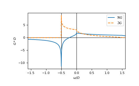
Local Green’s function of the 3D face-centered cubic (fcc) lattice.
Note, that the spectrum is asymmetric and in \([-D/2, 3D/2]\), where \(D\) is the half-bandwidth.
Has a van Hove singularity at z=-half_bandwidth/2 (divergence) and at z=0 (continuous but not differentiable).
Implements equations (2.16), (2.17) and (2.11) from [morita1971].
- Parameters:
- zcomplex np.ndarray or complex
Green’s function is evaluated at complex frequency z.
- half_bandwidthfloat
Half-bandwidth of the DOS of the face-centered cubic lattice. The half_bandwidth corresponds to the nearest neighbor hopping t=D/8.
- Returns:
- complex np.ndarray or complex
Value of the face-centered cubic lattice Green’s function.
References
[morita1971]Morita, T., Horiguchi, T., 1971. Calculation of the Lattice Green’s Function for the bcc, fcc, and Rectangular Lattices. Journal of Mathematical Physics 12, 986-992. https://doi.org/10.1063/1.1665693
Examples
>>> ww = np.linspace(-1.6, 1.6, num=501, dtype=complex)
>>> gf_ww = gt.lattice.fcc.gf_z(ww, half_bandwidth=1)
>>> import matplotlib.pyplot as plt
>>> _ = plt.axvline(-0.5, color='black', linewidth=0.8)
>>> _ = plt.axvline(0, color='black', linewidth=0.8)
>>> _ = plt.axhline(0, color='black', linewidth=0.8)
>>> _ = plt.plot(ww.real, gf_ww.real, label=r"$\Re G$")
>>> _ = plt.plot(ww.real, gf_ww.imag, '--', label=r"$\Im G$")
>>> _ = plt.ylabel(r"$G*D$")
>>> _ = plt.xlabel(r"$\omega/D$")
>>> _ = plt.xlim(left=ww.real.min(), right=ww.real.max())
>>> _ = plt.legend()
>>> plt.show()
