gftool.fourier.tt2z

gftool.fourier.tt2z(tt, gf_t, z, laplace=<function tt2z_lin>, **kwds)

Laplace transform of the real-time Green’s function gf_t.

Calculate the Laplace transform

\[G(z) = ∫dt G(t) \exp(izt)\]

For the Laplace transform to be well defined, it should either be tt>=0 and z.imag>=0 for the retarded Green’s function, or tt<=0 and z.imag<=0 for the advance Green’s function.

The retarded (advanced) Green’s function can in principle be evaluated for any frequency point z in the upper (lower) complex half-plane.

The accented contours for tt and z depend on the specific used back-end laplace.

Parameters:

tt(Nt) float np.ndarray

The points for which the Green’s function gf_t is given.

gf_t(…, Nt) complex np.ndarray

Green’s function at time points tt.

z(…, Nz) complex np.ndarray

Frequency points for which the Laplace transformed Green’s function should be evaluated.

laplace{tt2z_lin, tt2z_trapz, tt2z_pade, tt2z_herm2}, optional

Back-end to perform the actual Fourier transformation.

**kwds

Key-word arguments forwarded to laplace.

Returns:

(…, Nz) complex np.ndarray

Laplace transformed Green’s function for complex frequencies z.

Raises:

ValueError

If neither the condition for retarded or advanced Green’s function is fulfilled.

See also

tt2z_trapz

Back-end: approximate integral by trapezoidal rule.

tt2z_lin

Back-end: approximate integral by Filon’s method.

tt2z_pade

Back-end: use Fourier-Padé algorithm.

tt2z_herm2

Back-end: using square Hermite-Padé for Fourier.

Examples

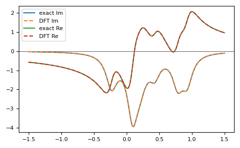
>>> tt = np.linspace(0, 150, num=1501)
>>> ww = np.linspace(-1.5, 1.5, num=501) + 1e-1j

>>> poles = 2*np.random.random(10) - 1  # partially filled
>>> weights = np.random.random(10)
>>> weights = weights/np.sum(weights)
>>> gf_ret_t = gt.pole_gf_ret_t(tt, poles=poles, weights=weights)
>>> gf_ft = gt.fourier.tt2z(tt, gf_ret_t, z=ww)
>>> gf_ww = gt.pole_gf_z(ww, poles=poles, weights=weights)

>>> import matplotlib.pyplot as plt
>>> __ = plt.axhline(0, color='dimgray', linewidth=0.8)
>>> __ = plt.plot(ww.real, gf_ww.imag, label='exact Im')
>>> __ = plt.plot(ww.real, gf_ft.imag, '--', label='DFT Im')
>>> __ = plt.plot(ww.real, gf_ww.real, label='exact Re')
>>> __ = plt.plot(ww.real, gf_ft.real, '--', label='DFT Re')
>>> __ = plt.legend()
>>> plt.tight_layout()
>>> plt.show()

(png, pdf)

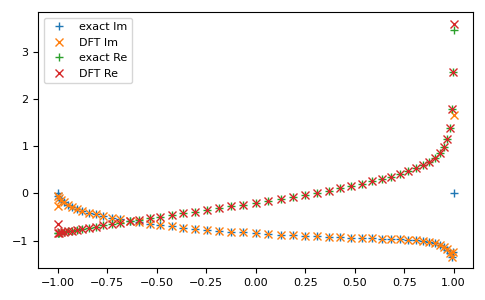
The function Laplace transform can be evaluated at abitrary contours, e.g. for a semi-ceircle in the the upper half-plane. Note, that close to the real axis the accuracy is bad, due to the truncation at max(tt)

>>> z = np.exp(1j*np.pi*np.linspace(0, 1, num=51))
>>> gf_ft = gt.fourier.tt2z(tt, gf_ret_t, z=z)
>>> gf_z = gt.pole_gf_z(z, poles=poles, weights=weights)

>>> import matplotlib.pyplot as plt
>>> __ = plt.plot(z.real, gf_z.imag, '+', label='exact Im')
>>> __ = plt.plot(z.real, gf_ft.imag, 'x', label='DFT Im')
>>> __ = plt.plot(z.real, gf_z.real, '+', label='exact Re')
>>> __ = plt.plot(z.real, gf_ft.real, 'x', label='DFT Re')
>>> __ = plt.legend()
>>> plt.tight_layout()
>>> plt.show()

(png, pdf)

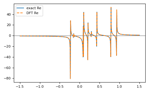
For small max(tt) close to the real axis, tt2z_pade is often the superior choice (it is taylored to resove poles):

>>> tt = np.linspace(0, 40, num=401)
>>> ww = np.linspace(-1.5, 1.5, num=501) + 1e-3j
>>> gf_ret_t = gt.pole_gf_ret_t(tt, poles=poles, weights=weights)
>>> gf_fp = gt.fourier.tt2z(tt, gf_ret_t, z=ww, laplace=gt.fourier.tt2z_pade)
>>> gf_ww = gt.pole_gf_z(ww, poles=poles, weights=weights)

>>> import matplotlib.pyplot as plt
>>> __ = plt.axhline(0, color='dimgray', linewidth=0.8)
>>> __ = plt.plot(ww.real, gf_ww.real, label='exact Re')
>>> __ = plt.plot(ww.real, gf_fp.real, '--', label='DFT Re')
>>> __ = plt.legend()
>>> plt.tight_layout()
>>> plt.show()

(png, pdf)

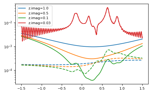
Accuracy of the different back-ends:

• For small z.imag or small tt[-1], tt2z_pade performs better than standard transformations tt2z_trapz and tt2z_lin. It is especially suited to resolve poles. For large tt.size, spurious features can appear.

• tt2z_herm2 further improves on tt2z_pade and can resolve square-root branch-cuts. Might be less stable as a wrong branch can be chosen.

• tt2z_trapz vs tt2z_lin:

  • For large z.imag, tt2z_lin performs better.

  • For intermediate z.imag, the quality depends on the relevant z.real. For small z.real, the error of tt2z_trapz is more uniform; for big z.real, tt2z_lin is a good approximation.

  • For small z.imag, the methods are almost identical, the truncation of tt dominates the error.

>>> tt = np.linspace(0, 150, num=1501)
>>> gf_ret_t = gt.pole_gf_ret_t(tt, poles=poles, weights=weights)
>>> import matplotlib.pyplot as plt
>>> for ii, eta in enumerate([1.0, 0.5, 0.1, 0.03]):
...     ww.imag = eta
...     gf_ww = gt.pole_gf_z(ww, poles=poles, weights=weights)
...     gf_trapz = gt.fourier.tt2z(tt, gf_ret_t, z=ww, laplace=gt.fourier.tt2z_trapz)
...     gf_lin = gt.fourier.tt2z(tt, gf_ret_t, z=ww, laplace=gt.fourier.tt2z_lin)
...     __ = plt.plot(ww.real, abs((gf_ww - gf_trapz)/gf_ww),
...                   label=f"z.imag={eta}", color=f"C{ii}")
...     __ = plt.plot(ww.real, abs((gf_ww - gf_lin)/gf_ww), '--', color=f"C{ii}")
...     __ = plt.legend()
>>> plt.yscale('log')
>>> plt.tight_layout()
>>> plt.show()

(png, pdf)