gftool.lattice.bcc.dos_mp

gftool.lattice.bcc.dos_mp(eps, half_bandwidth=1)

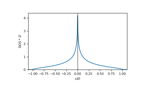
Multi-precision DOS of non-interacting 3D body-centered lattice.

Has a van Hove singularity (logarithmic divergence) at eps = 0.

This function is particularity suited to calculate integrals of the form \(∫dϵ DOS(ϵ)f(ϵ)\). If you have problems with the convergence, consider using \(∫dϵ DOS(ϵ)[f(ϵ)-f(0)] + f(0)\) to avoid the singularity.

Parameters:

epsmpmath.mpf or mpf_like

DOS is evaluated at points eps.

half_bandwidthmpmath.mpf or mpf_like

Half-bandwidth of the DOS, DOS(| eps | > half_bandwidth) = 0. The half_bandwidth corresponds to the nearest neighbor hopping t=D/8.

Returns:

mpmath.mpf

The value of the DOS.

See also

gftool.lattice.bcc.dos

Vectorized version suitable for array evaluations.

References

[morita1971]

Morita, T., Horiguchi, T., 1971. Calculation of the Lattice Green’s Function for the bcc, fcc, and Rectangular Lattices. Journal of Mathematical Physics 12, 986–992. https://doi.org/10.1063/1.1665693

Examples

Calculate integrals:

>>> from mpmath import mp
>>> mp.quad(gt.lattice.bcc.dos_mp, [-1, 0, 1])
mpf('1.0')

>>> eps = np.linspace(-1.1, 1.1, num=500)
>>> dos_mp = [gt.lattice.bcc.dos_mp(ee, half_bandwidth=1) for ee in eps]
>>> dos_mp = np.array(dos_mp, dtype=np.float64)

>>> import matplotlib.pyplot as plt
>>> _ = plt.plot(eps, dos_mp)
>>> _ = plt.xlabel(r"$\epsilon/D$")
>>> _ = plt.ylabel(r"DOS * $D$")
>>> _ = plt.axvline(0, color='black', linewidth=0.8)
>>> _ = plt.ylim(bottom=0)
>>> _ = plt.xlim(left=eps.min(), right=eps.max())
>>> plt.show()

(png, pdf)