gftool.lattice.rectangular.gf_z

gftool.lattice.rectangular.gf_z(z, half_bandwidth, scale)

Local Green’s function of the 2D rectangular lattice.

\[G(z) = \frac{1}{π} ∫_0^π \frac{dϕ}{\sqrt{(z - γ \cos ϕ)^2 - 1}}\]

where \(γ\) is the scale, the hopping is chosen t=1, the half_bandwidth is \(D=2(1+γ)\). The integral is the complete elliptic integral of first kind. See [morita1971].

Parameters:

zcomplex np.ndarray or complex

Green’s function is evaluated at complex frequency z.

half_bandwidthfloat

Half-bandwidth of the DOS of the rectangular lattice. The half_bandwidth corresponds to the nearest neighbor hopping \(t=D/2/(scale+1)\).

scalefloat

Relative scale of the different hoppings \(t_1=scale*t_2\). scale=1 corresponds to the square lattice.

Returns:

complex np.ndarray or complex

Value of the rectangular lattice Green’s function.

See also

gftool.lattice.square.gf_z

Green’s function in the limit scale=1.

References

[morita1971]

Morita, T., Horiguchi, T., 1971. Calculation of the Lattice Green’s Function for the bcc, fcc, and Rectangular Lattices. Journal of Mathematical Physics 12, 986–992. https://doi.org/10.1063/1.1665693

Examples

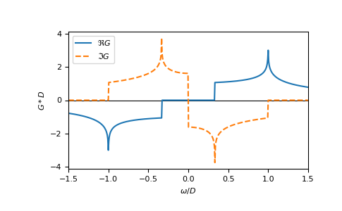
>>> ww = np.linspace(-1.5, 1.5, num=500, dtype=complex)
>>> gf_ww = gt.lattice.rectangular.gf_z(ww, half_bandwidth=1, scale=2)

>>> import matplotlib.pyplot as plt
>>> _ = plt.axhline(0, color='black', linewidth=0.8)
>>> _ = plt.plot(ww.real, gf_ww.real, label=r"$\Re G$")
>>> _ = plt.plot(ww.real, gf_ww.imag, '--', label=r"$\Im G$")
>>> _ = plt.ylabel(r"$G*D$")
>>> _ = plt.xlabel(r"$\omega/D$")
>>> _ = plt.xlim(left=ww.real.min(), right=ww.real.max())
>>> _ = plt.legend()
>>> plt.show()

(png, pdf)