gftool.polepade.continuation

gftool.polepade.continuation(z, fct_z, degree=-1, weight=None, moments=(), vandermond=<function polyvander>, rotate=None, real_asymp=True) → PadeApprox

Perform the Padé analytic continuation of (z, fct_z).

Parameters:

z, fct_z(N_z) complex np.ndarray

Variable where function is evaluated and function values.

degreeint, optional

The difference of denominator and numerator degree (default: -1). This determines how fct_z decays for large abs(z): fct_z → z**degree. For Green’s functions it typically is -1, for self-energies it typically is 0.

weight(N_z) float np.ndarray, optional

Weighting of the data points, for a known error σ this should be weight = 1./σ.

moments(N) float array_like

Moments of the high-frequency expansion, where f(z) = moments / z**np.arange(1, N+1) for large z. This only affects the calculated pade.residues, and constrains them to fulfill the moments.

Returns:

PadeApprox

Padé analytic continuation parametrized by pade.zeros, pade.poles and pade.residues.

Other Parameters:

vandermondCallable, optional

Function giving the Vandermond matrix of the chosen polynomial basis. Defaults to simple polynomials.

rotatebool or None, optional

Whether to rotate the coordinate to calculated zeros and poles (default: rotate if z is purely imaginary).

real_asympbool, optional

Whether to consider only the real part of the asymptote, or treat it as complex number. Physically, to asymptote should typically be real (default: True).

Examples

>>> beta = 100
>>> iws = gt.matsubara_frequencies(range(512), beta=beta)
>>> gf_iw = gt.square_gf_z(iws, half_bandwidth=1)
>>> weight = 1./iws.imag  # put emphasis on low frequencies
>>> gf_pade = gt.polepade.continuation(iws, gf_iw, weight=weight, moments=[1.])

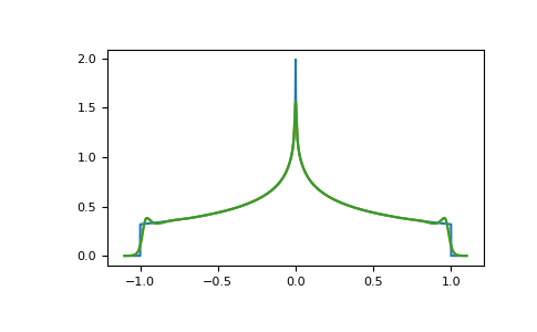
Compare the result on the real axis:

>>> import matplotlib.pyplot as plt
>>> ww = np.linspace(-1.1, 1.1, num=5000)
>>> __ = plt.plot(ww, gt.square_dos(ww, half_bandwidth=1))
>>> __ = plt.plot(ww, -1. / np.pi * gf_pade.eval_zeropole(ww).imag)
>>> __ = plt.plot(ww, -1. / np.pi * gf_pade.eval_polefct(ww).imag)
>>> plt.show()

(png, pdf)

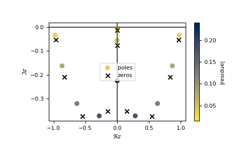
Investigate the pole structure of the continuation:

>>> gf_pade.plot()
>>> plt.show()

(png, pdf)