gftool.fourier.tau2iv
- gftool.fourier.tau2iv(gf_tau, beta, fourier=<function tau2iv_ft_lin>)[source]
Fourier transformation of the real Green’s function gf_tau.
Fourier transformation of a bosonic imaginary-time Green’s function to Matsubara domain. We assume a real Green’s function gf_tau, which is the case for commutator Green’s functions \(G_{AB}(τ) = ⟨A(τ)B⟩\) with \(A = B^†\). The Fourier transform gf_iv is then Hermitian. This function removes the discontinuity \(G_{AB}(β) - G_{AB}(0) = ⟨[A,B]⟩\).
TODO: if high-frequency moments are know, they should be stripped for increased accuracy.
- Parameters:
- gf_tau(…, N_tau) float np.ndarray
The Green’s function at imaginary times \(τ \in [0, β]\).
- betafloat
The inverse temperature \(beta = 1/k_B T\).
- fourier{
tau2iv_ft_lin,tau2iv_dft}, optional Back-end to perform the actual Fourier transformation.
- Returns:
- (…, (N_iv + 1)/2) complex np.ndarray
The Fourier transform of gf_tau for non-negative bosonic Matsubara frequencies \(iν_n\).
See also
tau2iv_dftBack-end: plain implementation using Riemann sum.
tau2iv_ft_linBack-end: Fourier integration using Filon’s method.
Examples
>>> BETA = 50
>>> tau = np.linspace(0, BETA, num=2049, endpoint=True)
>>> ivs = gt.matsubara_frequencies_b(range((tau.size+1)//2), beta=BETA)
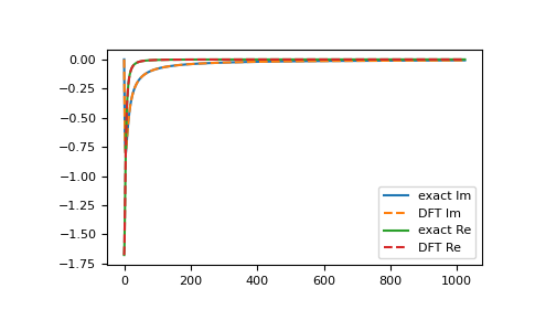
>>> poles, weights = np.random.random(10), np.random.random(10)
>>> weights = weights/np.sum(weights)
>>> gf_tau = gt.pole_gf_tau_b(tau, poles=poles, weights=weights, beta=BETA)
>>> gf_ft = gt.fourier.tau2iv(gf_tau, beta=BETA)
>>> gf_tau.size, gf_ft.size
(2049, 1025)
>>> gf_iv = gt.pole_gf_z(ivs, poles=poles, weights=weights)
>>> import matplotlib.pyplot as plt
>>> __ = plt.plot(gf_iv.imag, label='exact Im')
>>> __ = plt.plot(gf_ft.imag, '--', label='DFT Im')
>>> __ = plt.plot(gf_iv.real, label='exact Re')
>>> __ = plt.plot(gf_ft.real, '--', label='DFT Re')
>>> __ = plt.legend()
>>> plt.show()
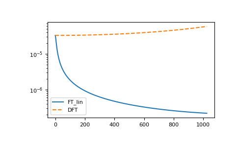
Accuracy of the different back-ends
>>> ft_lin, dft = gt.fourier.tau2iv_ft_lin, gt.fourier.tau2iv_dft
>>> gf_ft_lin = gt.fourier.tau2iv(gf_tau, beta=BETA, fourier=ft_lin)
>>> gf_dft = gt.fourier.tau2iv(gf_tau, beta=BETA, fourier=dft)
>>> __ = plt.plot(abs(gf_iv - gf_ft_lin), label='FT_lin')
>>> __ = plt.plot(abs(gf_iv - gf_dft), '--', label='DFT')
>>> __ = plt.legend()
>>> plt.yscale('log')
>>> plt.show()

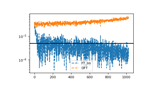
The methods are resistant against noise:
>>> magnitude = 5e-6
>>> noise = np.random.normal(scale=magnitude, size=gf_tau.size)
>>> gf_ft_lin_noisy = gt.fourier.tau2iv(gf_tau + noise, beta=BETA, fourier=ft_lin)
>>> gf_dft_noisy = gt.fourier.tau2iv(gf_tau + noise, beta=BETA, fourier=dft)
>>> __ = plt.plot(abs(gf_iv - gf_ft_lin_noisy), '--', label='FT_lin')
>>> __ = plt.plot(abs(gf_iv - gf_dft_noisy), '--', label='DFT')
>>> __ = plt.axhline(magnitude, color='black')
>>> __ = plt.legend()
>>> plt.yscale('log')
>>> plt.show()