gftool.fourier.tau2iw
- gftool.fourier.tau2iw(gf_tau, beta, n_pole=None, moments=None, fourier=<function tau2iw_ft_lin>)[source]
Fourier transform of the real Green’s function gf_tau.
Fourier transformation of a fermionic imaginary-time Green’s function to Matsubara domain. We assume a real Green’s function gf_tau, which is the case for commutator Green’s functions \(G_{AB}(τ) = ⟨A(τ)B⟩\) with \(A = B^†\). The Fourier transform gf_iw is then Hermitian. If no explicit moments are given, this function removes \(-G_{AB}(β) - G_{AB}(0) = ⟨[A,B]⟩\).
- Parameters:
- gf_tau(…, N_tau) float np.ndarray
The Green’s function at imaginary times \(τ \in [0, β]\).
- betafloat
The inverse temperature \(beta = 1/k_B T\).
- n_poleint, optional
Number of poles used to fit gf_tau. Needs to be at least as large as the number of given moments m (default: no fitting is performed).
- moments(…, m) float array_like, optional
High-frequency moments of gf_iw. If none are given, the first moment is chosen to remove the discontinuity at \(τ=0^{±}\).
- fourier{
tau2iw_ft_lin,tau2iw_dft}, optional Back-end to perform the actual Fourier transformation.
- Returns:
- (…, (N_iv + 1)/2) complex np.ndarray
The Fourier transform of gf_tau for non-negative fermionic Matsubara frequencies \(iω_n\).
See also
tau2iw_ft_linBack-end: Fourier integration using Filon’s method.
tau2iw_dftBack-end: plain implementation using Riemann sum.
pole_gf_from_tauFunction handling the fitting of gf_tau.
Examples
>>> BETA = 50
>>> tau = np.linspace(0, BETA, num=2049, endpoint=True)
>>> iws = gt.matsubara_frequencies(range((tau.size-1)//2), beta=BETA)
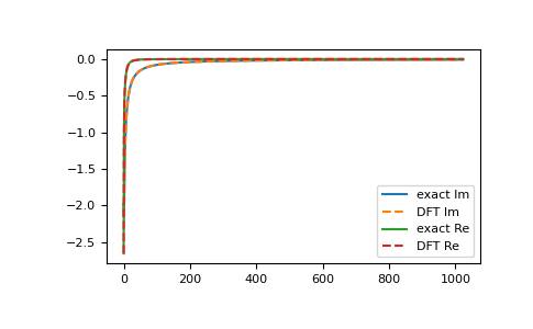
>>> poles = 2*np.random.random(10) - 1  # partially filled
>>> weights = np.random.random(10)
>>> weights = weights/np.sum(weights)
>>> gf_tau = gt.pole_gf_tau(tau, poles=poles, weights=weights, beta=BETA)
>>> gf_ft = gt.fourier.tau2iw(gf_tau, beta=BETA)
>>> gf_tau.size, gf_ft.size
(2049, 1024)
>>> gf_iw = gt.pole_gf_z(iws, poles=poles, weights=weights)
>>> import matplotlib.pyplot as plt
>>> __ = plt.plot(gf_iw.imag, label='exact Im')
>>> __ = plt.plot(gf_ft.imag, '--', label='DFT Im')
>>> __ = plt.plot(gf_iw.real, label='exact Re')
>>> __ = plt.plot(gf_ft.real, '--', label='DFT Re')
>>> __ = plt.legend()
>>> plt.show()

Accuracy of the different back-ends
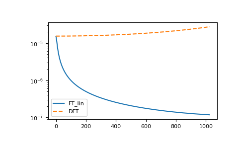
>>> ft_lin, dft = gt.fourier.tau2iw_ft_lin, gt.fourier.tau2iw_dft
>>> gf_ft_lin = gt.fourier.tau2iw(gf_tau, beta=BETA, fourier=ft_lin)
>>> gf_dft = gt.fourier.tau2iw(gf_tau, beta=BETA, fourier=dft)
>>> __ = plt.plot(abs(gf_iw - gf_ft_lin), label='FT_lin')
>>> __ = plt.plot(abs(gf_iw - gf_dft), '--', label='DFT')
>>> __ = plt.legend()
>>> plt.yscale('log')
>>> plt.show()

The accuracy can be further improved by fitting as suitable pole Green’s function:
>>> for n, n_mom in enumerate(range(1, 30, 5)):
...     gf = gt.fourier.tau2iw(gf_tau, n_pole=n_mom, moments=(1,), beta=BETA, fourier=ft_lin)
...     __ = plt.plot(abs(gf_iw - gf), label=f'n_fit={n_mom}', color=f'C{n}')
...     gf = gt.fourier.tau2iw(gf_tau, n_pole=n_mom, moments=(1,), beta=BETA, fourier=dft)
...     __ = plt.plot(abs(gf_iw - gf), '--', color=f'C{n}')
>>> __ = plt.legend(loc='lower right')
>>> plt.yscale('log')
>>> plt.show()
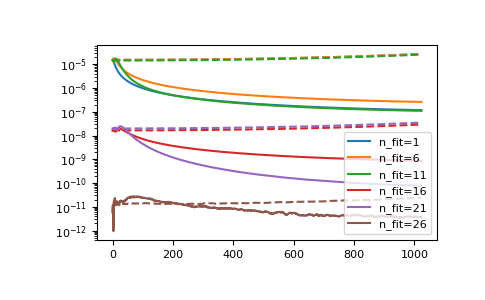
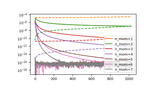
Results for DFT can be drastically improved giving high-frequency moments. The reason is, that lower large frequencies, where FT_lin is superior, are treated by the moments instead of the Fourier transform.
>>> mom = np.sum(weights[:, np.newaxis] * poles[:, np.newaxis]**range(8), axis=0)
>>> for n in range(1, 8):
...     gf = gt.fourier.tau2iw(gf_tau, moments=mom[:n], beta=BETA, fourier=ft_lin)
...     __ = plt.plot(abs(gf_iw - gf), label=f'n_mom={n}', color=f'C{n}')
...     gf = gt.fourier.tau2iw(gf_tau, moments=mom[:n], beta=BETA, fourier=dft)
...     __ = plt.plot(abs(gf_iw - gf), '--', color=f'C{n}')
>>> __ = plt.legend(loc='lower right')
>>> plt.yscale('log')
>>> plt.show()
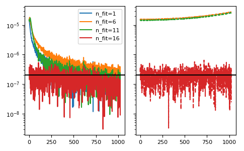
The method is resistant against noise:
>>> magnitude = 2e-7
>>> noise = np.random.normal(scale=magnitude, size=gf_tau.size)
>>> __, axes = plt.subplots(ncols=2, sharey=True)
>>> for n, n_mom in enumerate(range(1, 20, 5)):
...     gf = gt.fourier.tau2iw(gf_tau + noise, n_pole=n_mom, moments=(1,),
...                            beta=BETA, fourier=ft_lin)
...     __ = axes[0].plot(abs(gf_iw - gf), label=f'n_fit={n_mom}', color=f'C{n}')
...     gf = gt.fourier.tau2iw(gf_tau + noise, n_pole=n_mom, moments=(1,),
...                            beta=BETA, fourier=dft)
...     __ = axes[1].plot(abs(gf_iw - gf), '--', color=f'C{n}')
>>> for ax in axes:
...     __ = ax.axhline(magnitude, color='black')
>>> __ = axes[0].legend()
>>> plt.yscale('log')
>>> plt.tight_layout()
>>> plt.show()

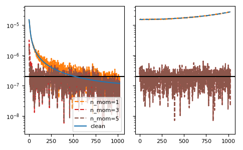
>>> __, axes = plt.subplots(ncols=2, sharey=True)
>>> for n in range(1, 7, 2):
...     gf = gt.fourier.tau2iw(gf_tau + noise, moments=mom[:n], beta=BETA, fourier=ft_lin)
...     __ = axes[0].plot(abs(gf_iw - gf), '--', label=f'n_mom={n}', color=f'C{n}')
...     gf = gt.fourier.tau2iw(gf_tau + noise, moments=mom[:n], beta=BETA, fourier=dft)
...     __ = axes[1].plot(abs(gf_iw - gf), '--', color=f'C{n}')
>>> for ax in axes:
...     __ = ax.axhline(magnitude, color='black')
>>> __ = axes[0].plot(abs(gf_iw - gf_ft_lin), label='clean')
>>> __ = axes[1].plot(abs(gf_iw - gf_dft), '--', label='clean')
>>> __ = axes[0].legend(loc='lower right')
>>> plt.yscale('log')
>>> plt.tight_layout()
>>> plt.show()
