gftool.fourier.tau2iw_dft
- gftool.fourier.tau2iw_dft(gf_tau, beta)[source]
Discrete Fourier transform of the real Green’s function gf_tau.
Fourier transformation of a fermionic imaginary-time Green’s function to Matsubara domain. The Fourier integral is replaced by a Riemann sum giving a discrete Fourier transform (DFT). We assume a real Green’s function gf_tau, which is the case for commutator Green’s functions \(G_{AB}(τ) = ⟨A(τ)B⟩\) with \(A = B^†\). The Fourier transform gf_iw is then Hermitian.
- Parameters:
- gf_tau(…, N_tau) float np.ndarray
The Green’s function at imaginary times \(τ \in [0, β]\).
- betafloat
The inverse temperature \(beta = 1/k_B T\).
- Returns:
- (…, (N_iw - 1)/2) float np.ndarray
The Fourier transform of gf_tau for positive fermionic Matsubara frequencies \(iω_n\).
See also
tau2iw_ft_linFourier integration using Filon’s method.
Examples
>>> BETA = 50
>>> tau = np.linspace(0, BETA, num=2049, endpoint=True)
>>> iws = gt.matsubara_frequencies(range((tau.size-1)//2), beta=BETA)
>>> poles = 2*np.random.random(10) - 1  # partially filled
>>> weights = np.random.random(10)
>>> weights = weights/np.sum(weights)
>>> gf_tau = gt.pole_gf_tau(tau, poles=poles, weights=weights, beta=BETA)
>>> # 1/z tail has to be handled manually
>>> gf_dft = gt.fourier.tau2iw_dft(gf_tau + .5, beta=BETA) + 1/iws
>>> gf_tau.size, gf_dft.size
(2049, 1024)
>>> gf_iw = gt.pole_gf_z(iws, poles=poles, weights=weights)
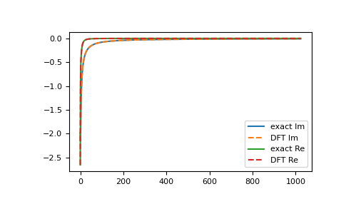
>>> import matplotlib.pyplot as plt
>>> __ = plt.plot(gf_iw.imag, label='exact Im')
>>> __ = plt.plot(gf_dft.imag, '--', label='DFT Im')
>>> __ = plt.plot(gf_iw.real, label='exact Re')
>>> __ = plt.plot(gf_dft.real, '--', label='DFT Re')
>>> __ = plt.legend()
>>> plt.show()

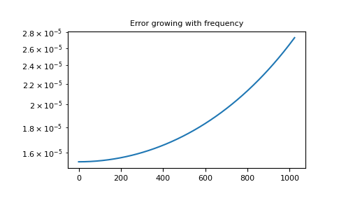
>>> __ = plt.title('Error growing with frequency')
>>> __ = plt.plot(abs(gf_iw - gf_dft))
>>> plt.yscale('log')
>>> plt.show()

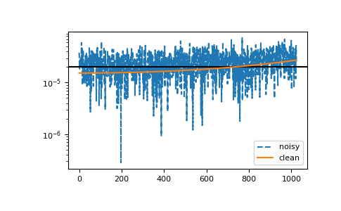
The method is resistant against noise:
>>> magnitude = 2e-5
>>> noise = np.random.normal(scale=magnitude, size=gf_tau.size)
>>> gf_dft_noisy = gt.fourier.tau2iw_dft(gf_tau + noise + .5, beta=BETA) + 1/iws
>>> __ = plt.plot(abs(gf_iw - gf_dft_noisy), '--', label='noisy')
>>> __ = plt.axhline(magnitude, color='black')
>>> __ = plt.plot(abs(gf_iw - gf_dft), label='clean')
>>> __ = plt.legend()
>>> plt.yscale('log')
>>> plt.show()